Complex Beam Propagation
To demonstrate the full power of HankelTransform with complex values, we will give an example of propagating a radially-symmetric beam using the beam propagation method.
In this case, it will be a simple Gaussian beam propagating away from focus and diverging. We'll utilize the <T: HankelScalar> generic trait to perform the QDHT directly on a Complex64 array.
First we will use a loop over the \(z\) position, and then we will demonstrate that the HankelTransform methods can perfectly vectorize the \(z\)-axis propagation by processing multiple columns natively.
Here is the source code:
mod helper;
use hankrs::HankelTransform;
use ndarray::{Array1, Array2, Axis};
use num_complex::Complex64;
use std::f64::consts::PI;

use crate::helper::{imagesc, plot_1d, plot_1d_compare};

#[allow(clippy::too_many_lines, clippy::similar_names)]
fn main() -> Result<(), Box<dyn std::error::Error>> {
    let nr = 1024;
    let r_max = 5e-3;
    let r = Array1::linspace(0.0, r_max, nr);

    let nz = 200;
    let z_max = 0.1;
    let z = Array1::linspace(0.0, z_max, nz);

    let dr = 100e-6;
    let lambda_ = 488e-9;
    let k0 = 2.0 * PI / lambda_;

    // Set up a HankelTransform object, telling it the order (0) and the radial grid.
    let transformer = HankelTransform::new_from_r_grid(0, r.clone()).unwrap();

    // Set up the electric field profile at z = 0, and resample onto the correct radial grid
    // (transformer.radius()) as required for the QDHT.
    let er_real = helper::gauss1d(&r, 0.0, dr);
    let er: Array1<Complex64> = er_real.mapv(|v| Complex64::new(v, 0.0));
    let er_h = transformer.to_transform_r(&er).unwrap();

    // Convert from physical field to physical wavevector
    let ekr_h = transformer.qdht(&er_h, Axis(0));

    // Plotting
    // Plot the initial field and radial wavevector distribution (given by the
    // Hankel transform)

    let r_mm = r.mapv(|val| val * 1e3);
    let transformer_r_mm = transformer.radius().mapv(|val| val * 1e3);

    let abs_er = er.mapv(|c| c.norm_sqr());
    let abs_er_h = er_h.mapv(|c| c.norm_sqr());

    plot_1d_compare(
        "usage_example_initial_field.png",
        &r_mm,
        &abs_er,
        &transformer_r_mm,
        &abs_er_h,
        "|E(r)|^2",
        "|E(H.r)|^2",
        "Initial electric field distribution",
        "Radial co-ordinate (r) /mm",
        "Field intensity /arb.",
        0.0..1.0,
        0.0..1.0,
    )?;

    let abs_ekr_h = ekr_h.mapv(|c| c.norm_sqr());
    let ht_max = abs_ekr_h.iter().copied().fold(f64::NEG_INFINITY, f64::max);
    plot_1d(
        "usage_example_k_vector.png",
        &transformer.kr(),
        &abs_ekr_h,
        "Radial wave-vector distribution",
        "Radial wave-vector (k_r) /rad m^-1",
        "Field intensity /arb.",
        0.0..30000.0,
        0.0..ht_max * 1.05,
    )?;

    // Propagate the beam - loop
    // Do the propagation in a loop over z
    // Pre-allocate an array for field as a function of r and z
    let mut erz = Array2::<Complex64>::zeros((nr, nz));
    let kz = transformer
        .kr()
        .mapv(|kr_val| (k0 * k0 - kr_val * kr_val).sqrt());

    for (i, &z_loop) in z.iter().enumerate() {
        let phi_z = kz.mapv(|kz_val| kz_val * z_loop); // Propagation phase
        let ekr_hz = ndarray::Zip::from(&ekr_h)
            .and(&phi_z)
            .map_collect(|&ekr, &phi| ekr * Complex64::new(0.0, phi).exp()); // Apply propagation
        let er_hz = transformer.iqdht(&ekr_hz, Axis(0)); // iQDHT
        let erz_slice = transformer.to_original_r(&er_hz).unwrap(); // Interpolate output
        erz.column_mut(i).assign(&erz_slice);
    }
    let irz = erz.mapv(|c| c.norm_sqr());

    let z_mm = z.mapv(|val| val * 1e3);
    let r_mm = r.mapv(|val| val * 1e3);

    // Now plot an image showing the intensity as a function of
    // radius and propagation distance.

    imagesc(
        "usage_example_irz.png",
        &z_mm,
        &r_mm,
        &irz,
        "Radial field intensity",
        "Propagation distance (z) /mm",
        "Radial position (r) /mm",
        0.0..1.0,
    )?;

    // The plot above shows a reduction of intensity with z, but it is
    // bit difficult to see the beam growing in r. To show that, let's
    // plot the intensity normalised such that the peak intensity at each z
    // coordinate is the same.
    let mut irz_norm = irz.clone();
    for i in 0..nz {
        let peak = irz_norm
            .column(i)
            .iter()
            .copied()
            .fold(f64::NEG_INFINITY, f64::max);
        if peak > 0.0 {
            let mut col = irz_norm.column_mut(i);
            col.mapv_inplace(|v| v / peak);
        }
    }

    imagesc(
        "usage_example_irz_norm.png",
        &z_mm,
        &r_mm,
        &irz_norm,
        "Normalised Radial field intensity",
        "Propagation distance (z) /mm",
        "Radial position (r) /mm",
        0.0..1.0,
    )?;

    // Propagate the beam - vectorised approach
    // We can also propagate it entirely within Hankel space without having to drop out in a loop!
    // By creating a 2D array of the wave propagation, we can apply the inverse QDHT
    // down the 0th axis in a single vectorized shot.
    let ekr_hz_vec = Array2::from_shape_fn((nr, nz), |(i, j)| {
        ekr_h[i] * Complex64::new(0.0, kz[i] * z[j]).exp()
    });

    let er_hz_vec = transformer.iqdht(&ekr_hz_vec, Axis(0));
    let erz_vec = transformer.to_original_r_nd(&er_hz_vec, Axis(0)).unwrap();

    let irz_vec = erz_vec.mapv(|c| c.norm_sqr());

    // Now plot the result to check it is the same as the loop approach
    imagesc(
        "usage_example_irz_vec.png",
        &z_mm,
        &r_mm,
        &irz_vec,
        "Radial field intensity as a function of propagation for annular beam",
        "Propagation distance (z) /mm",
        "Radial position (r) /mm",
        0.0..1.0,
    )?;

    #[allow(clippy::cast_precision_loss)]
    let total_n = (nr * nz) as f64;
    // Assert the two approaches produce the same intensity
    // Assert matches
    let error: f64 = irz
        .iter()
        .zip(irz_vec.iter())
        .map(|(&a, &b)| (a - b).abs())
        .sum::<f64>()
        / total_n;
    assert!(error < 1e-10);

    Ok(())
}
Initial Electric Field Distribution:
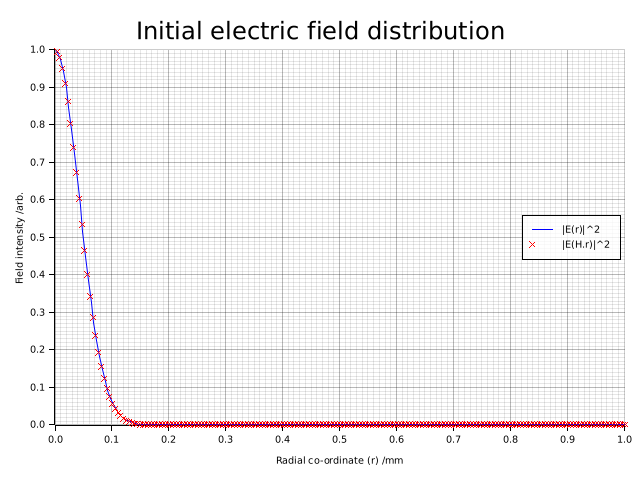
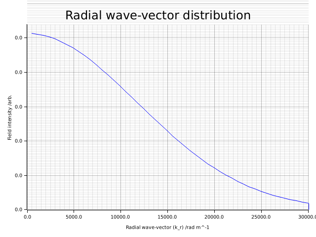
Radial Field Intensity as a Function of Propagation:
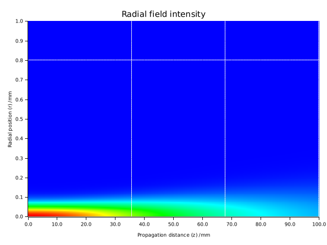
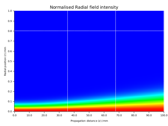
Because the intensity drops as the beam expands, it might be difficult to clearly see the beam growing in \(r\). To show that better, let's plot the intensity normalised such that the peak intensity at each \(z\) coordinate is identical.
Normalised Radial Field Intensity:
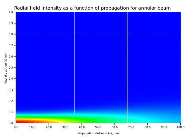
Vectorised Approach Match:
We can also verify that propagating it using the vectorised array matches the loop exactly.