Literature Comparison
This example is a comparison of hankrs against results from the original publication of the quasi-discrete Hankel transform method:
"Computation of quasi-discrete Hankel transforms of the integer order for propagating optical wave fields" Manuel Guizar-Sicairos and Julio C. Guitierrez-Vega J. Opt. Soc. Am. A 21 (1) 53-58 (2004)
mod helper;
use amos_bessel_rs::bessel_j;
use approx::assert_abs_diff_eq;
use hankrs::HankelTransform;
use ndarray::{Array1, ArrayRef1, Axis};
use std::f64::consts::PI;

use crate::helper::{plot_1d, plot_1d_compare};

fn sinc(x: &ArrayRef1<f64>) -> Array1<f64> {
    x.mapv(|val| if val == 0.0 { 1.0 } else { val.sin() / val })
}

/// Equation 12 of Guizar
fn hankel_transform_of_sinc(v: &ArrayRef1<f64>, gamma: f64, p: i32) -> Array1<f64> {
    v.mapv(|val| {
        if val < gamma {
            val.powi(p) * (f64::from(p) * PI / 2.0).cos()
                / (2.0
                    * PI
                    * gamma
                    * (gamma * gamma - val * val).sqrt()
                    * (gamma + (gamma * gamma - val * val).sqrt()).powi(p))
        } else {
            (f64::from(p) * (gamma / val).asin()).sin()
                / (2.0 * PI * gamma * (val * val - gamma * gamma).sqrt())
        }
    })
}

#[allow(clippy::cast_precision_loss, clippy::too_many_lines)]
fn main() -> Result<(), Box<dyn std::error::Error>> {
    // 1. Sinc function and dynamical error (Figure 1 of Guizar)
    // First we will reproduce figure 1 of Guizar-Sicairos & Guitierrez-Vega
    // Now plot the values of the hankel transform and the dynamical error as in figure 1
    // for order 1 and 4
    for &p in &[1, 4] {
        let transformer = HankelTransform::new(p, 3.0, 256).unwrap();
        let gamma = 5.0;
        let r = transformer.radius();
        let func = sinc(&r.mapv(|rad| 2.0 * PI * gamma * rad));
        let v = transformer.kr().mapv(|k| k / (2.0 * PI));
        let expected_ht = hankel_transform_of_sinc(&v, gamma, p);
        let ht = transformer.qdht(&func, Axis(0));

        let v_linear = Array1::linspace(0.0, 10.0, 1024);
        let expected_ht_linear = hankel_transform_of_sinc(&v_linear, gamma, p);

        let ht_max = ht.iter().copied().fold(f64::NEG_INFINITY, f64::max);
        let dynamical_error = ht
            .iter()
            .zip(expected_ht.iter())
            .map(|(&h, &e)| 20.0 * ((e - h).abs() / ht_max).log10())
            .collect::<Array1<f64>>();

        let title = format!("Hankel Transform, p={p}");
        plot_1d_compare(
            &format!("lit_comp_sinc_ht_{p}.png"),
            &v_linear,
            &expected_ht_linear,
            &v,
            &ht,
            "Analytical",
            "QDHT",
            &title,
            "Frequency /v",
            "Amplitude",
            0.0..10.0,
            -0.05..0.05,
        )?;

        plot_1d(
            &format!("lit_comp_sinc_error_{p}.png"),
            &v,
            &dynamical_error,
            "Dynamical error",
            "Frequency /v",
            "Error /dB",
            0.0..10.0,
            -150.0..0.0,
        )?;
    }

    // 2. Figure 3 and Table 1 of Guizar
    // Now we will reproduce figure 3 and confirm we can replicate
    // the errors in the top half of table 1.
    let p = 4;
    let a = 1.0;

    // We'll just do 1024 points for the example
    let transformer = HankelTransform::new(p, 2.0, 1024).unwrap();
    let r = transformer.radius();
    let func = r.mapv(|rad| if rad <= a { rad.powi(p) } else { 0.0 });

    let v = transformer.kr().mapv(|k| k / (2.0 * PI));
    let expected_ht = v.mapv(|v_val| {
        if v_val == 0.0 {
            0.0 // handled implicitly in jinc
        } else {
            a.powi(p + 1) * bessel_j(f64::from(p) + 1.0, 2.0 * PI * a * v_val).unwrap() / v_val
        }
    });

    let v_linear = Array1::linspace(0.0, 10.0, 1024);
    let expected_ht_linear = v_linear.mapv(|v_val| {
        if v_val == 0.0 {
            0.0 // handled implicitly in jinc
        } else {
            a.powi(p + 1) * bessel_j(f64::from(p) + 1.0, 2.0 * PI * a * v_val).unwrap() / v_val
        }
    });

    let ht = transformer.qdht(&func, Axis(0));
    let retrieved_func = transformer.iqdht(&ht, Axis(0));

    let v = transformer.kr().mapv(|k| k / (2.0 * PI));
    plot_1d_compare(
        "lit_comp_fig3_ht.png",
        &v_linear,
        &expected_ht_linear,
        &v,
        &ht,
        "Analytical",
        "QDHT",
        &format!("Hankel transform f_2(v), order {p}"),
        "Frequency /v",
        "Amplitude",
        0.0..10.0,
        -0.2..1.0,
    )?;

    let r_linear = Array1::linspace(0.0, 2.0, 1024);
    let func_linear = r_linear.mapv(|rad| if rad <= a { rad.powi(p) } else { 0.0 });

    plot_1d_compare(
        "lit_comp_fig3_retrieved.png",
        &r_linear,
        &func_linear,
        &r,
        &retrieved_func,
        "Analytical",
        "QDHT+iQDHT",
        "Round-trip QDHT vs analytical function",
        "Radius /r",
        "Amplitude",
        0.0..2.0,
        -0.2..1.2,
    )?;

    // Now check that the error is the same as that given in Table 1
    // Check that the error is low, as they do in the paper. Numbers are estimated from their graphs
    let error_2: f64 = expected_ht
        .iter()
        .zip(ht.iter())
        .map(|(&e, &h)| (e - h).abs())
        .sum::<f64>()
        / ht.len() as f64;
    let error_1: f64 = func
        .iter()
        .zip(retrieved_func.iter())
        .map(|(&f_val, &r_val)| (f_val - r_val).abs())
        .sum::<f64>()
        / func.len() as f64;

    println!("**1024 Points:**");
    println!("- Error in Hankel transform is {error_2:.2e}");
    println!("- Error in reconstructed function is {error_1:.2e}");

    assert_abs_diff_eq!(error_2, 4.8e-5, epsilon = 1e-6);
    // Note that Guizar-Sicairos & Guitierrez-Vega got 2.7e-14, so ours is slightly lower
    assert_abs_diff_eq!(error_1, 2.15e-14, epsilon = 1e-15);

    // Now repeat for 512 points
    let transformer_512 = HankelTransform::new(p, 2.0, 512).unwrap();
    let r_512 = transformer_512.radius();
    let func_512 = r_512.mapv(|rad| if rad <= a { rad.powi(p) } else { 0.0 });

    let v_512 = transformer_512.kr().mapv(|k| k / (2.0 * PI));
    let expected_ht_512 = v_512.mapv(|v_val| {
        if v_val == 0.0 {
            0.0 // handled implicitly in jinc
        } else {
            a.powi(p + 1) * bessel_j(f64::from(p) + 1.0, 2.0 * PI * a * v_val).unwrap() / v_val
        }
    });

    let ht_512 = transformer_512.qdht(&func_512, Axis(0));
    let retrieved_func_512 = transformer_512.iqdht(&ht_512, Axis(0));

    let error_2_512: f64 = expected_ht_512
        .iter()
        .zip(ht_512.iter())
        .map(|(&e, &h)| (e - h).abs())
        .sum::<f64>()
        / ht_512.len() as f64;
    let error_1_512: f64 = func_512
        .iter()
        .zip(retrieved_func_512.iter())
        .map(|(&f_val, &r_val)| (f_val - r_val).abs())
        .sum::<f64>()
        / func_512.len() as f64;

    println!("\n**512 Points:**");
    println!("- Error in Hankel transform is {error_2_512:.2e}");
    println!("- Error in reconstructed function is {error_1_512:.2e}");

    // Note the below is 10 times smaller than
    // Guizar-Sicairos & Guitierrez-Vega (1.3e-3)
    assert_abs_diff_eq!(error_2_512, 1.3e-4, epsilon = 1e-5);
    assert_abs_diff_eq!(error_1_512, 2.2e-13, epsilon = 1e-14);

    Ok(())
}
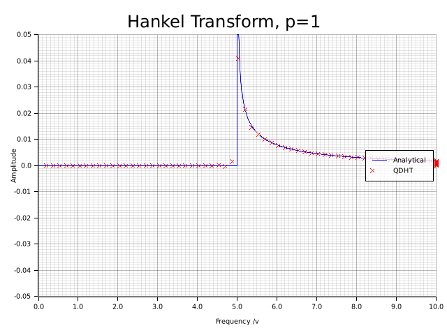
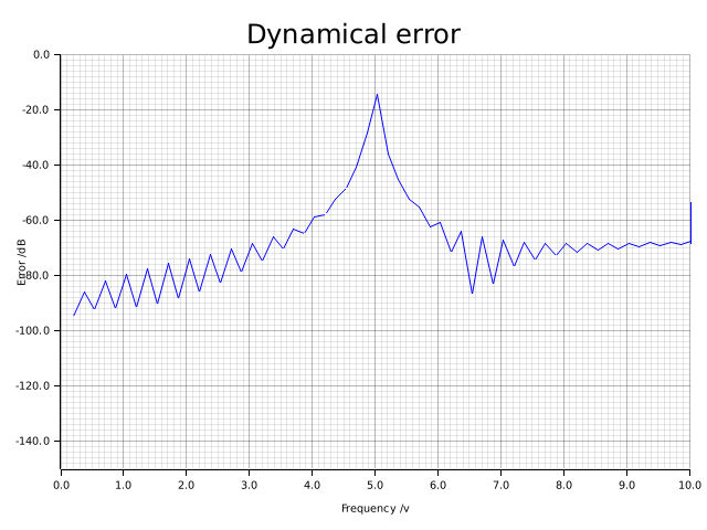
Figure 1: Hankel Transform of a Sinc Function
We reproduce figure 1 of Guizar-Sicairos & Guitierrez-Vega, showing the Hankel transform of a sinc function and the dynamical error, for orders 1 and 4.
Order 1
Order 4
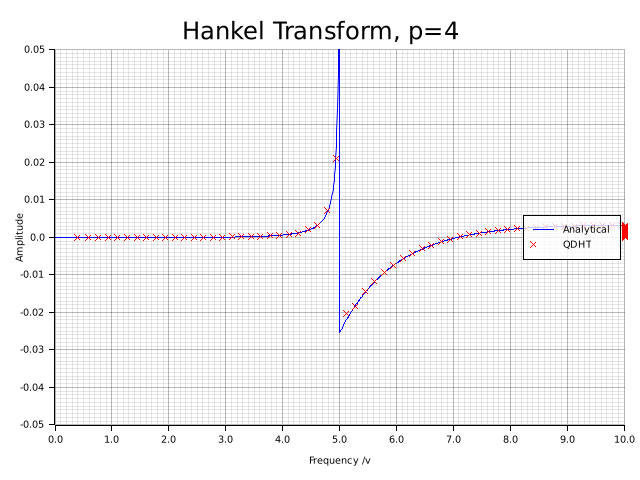
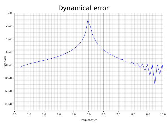
Figure 3: Round-Trip Transformation
We reproduce figure 3, applying a forward transform and an inverse transform (round-trip), demonstrating high fidelity.
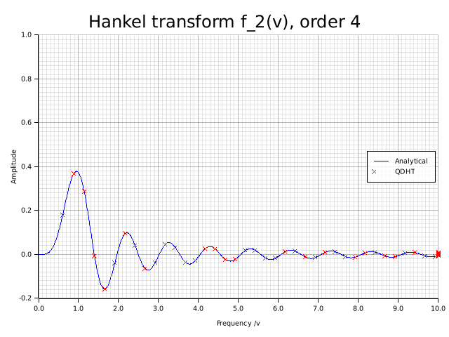
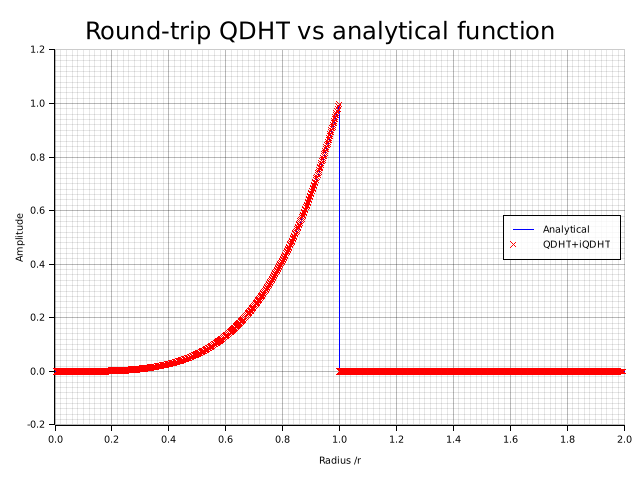
Table 1: Error Calculations
The calculated errors for the Hankel transform and the reconstructed function match the values given in Table 1 of the Guizar-Sicairos & Guitierrez-Vega paper.
1024 Points:
- Error in Hankel transform is 4.81e-5
- Error in reconstructed function is 2.12e-14
512 Points:
- Error in Hankel transform is 1.35e-4
- Error in reconstructed function is 2.26e-13