Known Transforms — Spherical Hankel Transform
The spherical Hankel transform (SQDHT) is a variant of the QDHT designed for functions with spherical (3-D radial) symmetry. It computes
$$ H_\text{sph}^{(n)}{f}(k) = \int_0^\infty f(r)\; j_n(kr) \; r^2 \; dr $$
where \(j_n(x)\) is the nth-order spherical Bessel function of the first kind, defined as
$$ j_n(x) = \sqrt{\frac{\pi}{2x}} \; J_{n+\frac{1}{2}}(x) $$
Where \(J_n(x)\) is the Bessel function of the first kind. For n = 0, this reduces to \(j_0(x) = \sin(x)/x\) and hence
$$ H_\text{sph}^{(0)}{f}(k) = \int_0^\infty f(r) \, \frac{\sin(kr)}{kr} \, r^2 \, dr $$
While the zeroth order transform is demonstrated below, the HankelTransform object can be used to compute
transforms of any integer order.
A HankelTransform configured for spherical symmetry can be created with
HankelTransform::new_spherical(order, max_radius, n_points).
Below we verify two well-known transform pairs against their analytical results.
mod helper;

use hankrs::HankelTransform;
use helper::plot_1d_original_and_transform;
use ndarray::{Array1, Axis};
use std::f64::consts::PI;

fn main() -> Result<(), Box<dyn std::error::Error>> {
    // 1. Spherical Gaussian transform
    //
    // The order-0 spherical Hankel transform of a Gaussian f(r) = exp(-a*r^2) has the
    // analytical result:
    //
    //   H_sph{ f(r) }(k) = (sqrt(pi) / (4 * a^(3/2))) * exp(-k^2 / (4a))
    //
    // We demonstrate this for a = 2.0.
    let a = 2.0_f64;
    let r_max = 20.0;
    let n_points = 250;

    let transformer = HankelTransform::new_spherical(0, r_max, n_points).unwrap();

    let function: Array1<f64> = transformer.radius().mapv(|r| (-a * r.powi(2)).exp());

    let actual_transform = transformer.qdht(&function, Axis(0));
    let kr = transformer.kr();

    // Dense analytical curve for plotting
    let kr_linear = Array1::linspace(0.0, *kr.last().unwrap(), 1024);
    let expected_transform = kr_linear.mapv(|k| {
        let prefactor = PI.sqrt() / (4.0 * a.powf(1.5));
        prefactor * (-(k.powi(2)) / (4.0 * a)).exp()
    });

    // Dense original function for plotting
    let r_linear = Array1::linspace(0.0, r_max * 0.5, 1024);
    let f_linear = r_linear.mapv(|r| (-a * r.powi(2)).exp());

    plot_1d_original_and_transform(
        "spherical_known_transforms_gaussian.png",
        &r_linear,
        &f_linear,
        "Gaussian function: exp(-r²)",
        "Radius r",
        "Amplitude",
        0.0..4.0,
        -0.05..1.05,
        &kr_linear,
        &expected_transform,
        &kr,
        &actual_transform,
        "Analytical",
        "SQDHT",
        "Spherical Hankel transform - Gaussian",
        "Wavenumber k",
        "Amplitude",
        0.0..10.0,
        -0.01..0.2,
    )?;

    // 2. Spherical top-hat transform
    //
    // The order-0 spherical Hankel transform of a top-hat function f(r) = 1 for r < a,
    // 0 otherwise, has the analytical result:
    //
    //   H_sph{ f(r) }(k) = (sin(ka) - ka*cos(ka)) / k^3
    //
    // We demonstrate this for a = 0.5
    let a_hat = 0.5_f64;
    let r_max_hat = 20.0;
    let n_points_hat = 1000;

    let transformer_hat = HankelTransform::new_spherical(0, r_max_hat, n_points_hat).unwrap();

    // Build top-hat on the QDHT grid; snap `a` to the nearest grid point
    let function_hat: Array1<f64> = transformer_hat
        .radius()
        .mapv(|r| if r < a_hat { 1.0 } else { 0.0 });

    // Snap a to the nearest grid sample to remove discretisation error in the comparison
    let actual_a = transformer_hat
        .radius()
        .iter()
        .rposition(|&r| r < a_hat)
        .map_or(a_hat, |idx| transformer_hat.radius()[idx]);

    let actual_transform_hat = transformer_hat.qdht(&function_hat, Axis(0));
    let kr_hat = transformer_hat.kr();

    // Dense analytical curve for plotting
    let kr_hat_linear = Array1::linspace(1e-6, *kr_hat.last().unwrap(), 1024);
    let expected_transform_hat = kr_hat_linear
        .mapv(|k| { (k * actual_a).sin() - k * actual_a * (k * actual_a).cos() } / k.powi(3));

    // Dense original function for plotting
    let r_hat_linear = Array1::linspace(0.0, 3.0, 1024);
    let f_hat_linear = r_hat_linear.mapv(|r| if r < a_hat { 1.0 } else { 0.0 });

    plot_1d_original_and_transform(
        "spherical_known_transforms_tophat.png",
        &r_hat_linear,
        &f_hat_linear,
        "Top-hat function: 1 for r < a",
        "Radius r",
        "Amplitude",
        0.0..2.0,
        -0.1..1.2,
        &kr_hat_linear,
        &expected_transform_hat,
        &kr_hat,
        &actual_transform_hat,
        "Analytical",
        "SQDHT",
        "Spherical Hankel transform - Top-Hat",
        "Wavenumber k",
        "Amplitude",
        0.0..30.0,
        -0.02..0.05,
    )?;

    Ok(())
}
Gaussian Function
The order-0 spherical Hankel transform of the Gaussian \(f(r) = e^{-ar^2}\) is
$$H_\text{sph}{e^{-ar^2}}(k) = \frac{\sqrt{\pi}}{4\, a^{3/2}}\, e^{-k^2 / 4a}$$
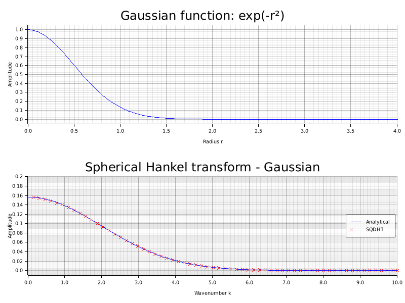
The SQDHT (circles) closely follows the analytical result (solid line) across the entire wavenumber range.
Top-Hat Function
The order-0 spherical Hankel transform of the top-hat \(f(r) = 1\) for \(r < a\), \(0\) otherwise, is
$$H_\text{sph}{f}(k) = \frac{\sin(ka) - ka\cos(ka)}{k^3}$$
This is the 3-D analogue of the familiar jinc function that arises in the standard (2-D radially-symmetric) Hankel transform.
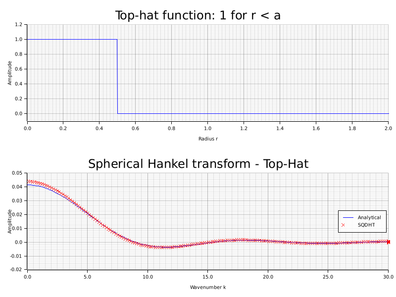
The oscillatory decay of the transform reflects the sharp edge of the top-hat, again in excellent agreement with the analytical formula.