hankrs
hankrs is a Rust implementation of the quasi-discrete Hankel transform. It was designed for use primarily in cases where a discrete Hankel transform is required, similar to the FFT for a Fourier transform.
Example Gallery
This documentation hosts a gallery of usage examples demonstrating the capabilities, speed, and accuracy of hankrs.
Use the sidebar to navigate through the gallery and see hankrs in action. All plots and outputs shown in the examples are generated directly by the underlying Rust code.
Simple Example
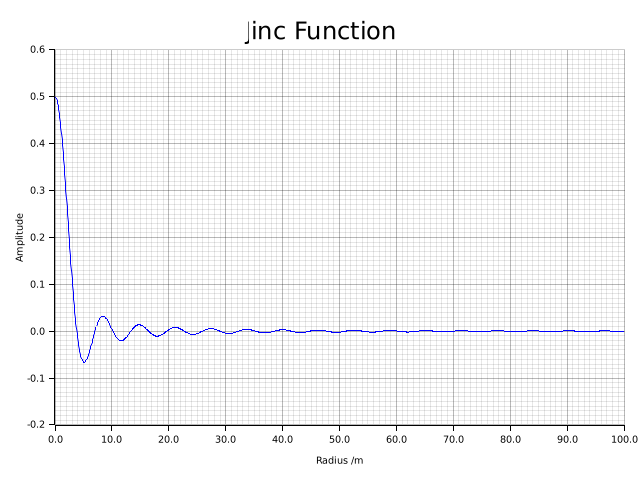
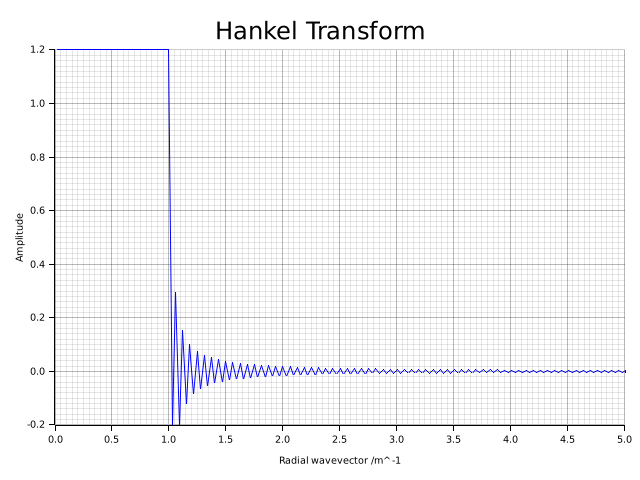
In this example (as in the One-Shot Example) we will check the band limit of a jinc function: \(f(r) = \frac{J_1(r)}{r}\). The (0 order) Hankel transform of this should be the top hat function.
Here we create a HankelTransform object and use its qdht method.
In this simple case, the simpler, single shot functions used in the One-Shot Example may be simpler to use. It should be noted, however, that they are not well suited for multiple transforms on the same grid and the approach taken here is recommended.
Here is the source code:
mod helper;
use amos_bessel_rs::bessel_j;
use hankrs::HankelTransform;
use ndarray::Axis;

use crate::helper::plot_1d;

fn main() -> Result<(), Box<dyn std::error::Error>> {
    // Create a HankelTransform object which holds the grid for r and kr points.
    let transformer = HankelTransform::new(0, 100.0, 1024).unwrap();
    let radius = transformer.radius();

    // Note that although the calculation fails at r = 0, transformer.radius() does not include r=0.
    let f = radius.mapv(|rad| bessel_j(1.0, rad).unwrap() / rad);

    plot_1d(
        "simple_example_f.png",
        &radius,
        &f,
        "Jinc Function",
        "Radius /m",
        "Amplitude",
        0.0..100.0,
        -0.2..0.6,
    )?;

    // Now take the Hankel transform using transformer.qdht
    let ht = transformer.qdht(&f, Axis(0));

    // As expected, this is a top-hat function bandlimited to k<1, except for numerical error.
    plot_1d(
        "simple_example_ht.png",
        &transformer.kr(),
        &ht,
        "Hankel Transform",
        "Radial wavevector /m^-1",
        "Amplitude",
        0.0..5.0,
        -0.2..1.2,
    )?;

    Ok(())
}
Original Function:
Hankel Transform (QDHT):
One-Shot Example
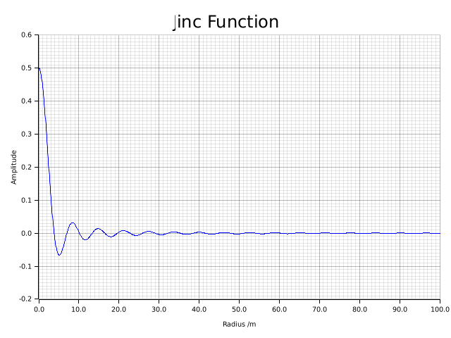
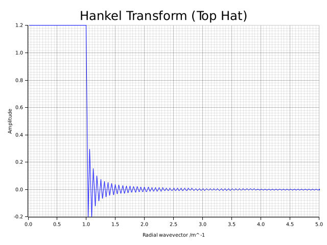
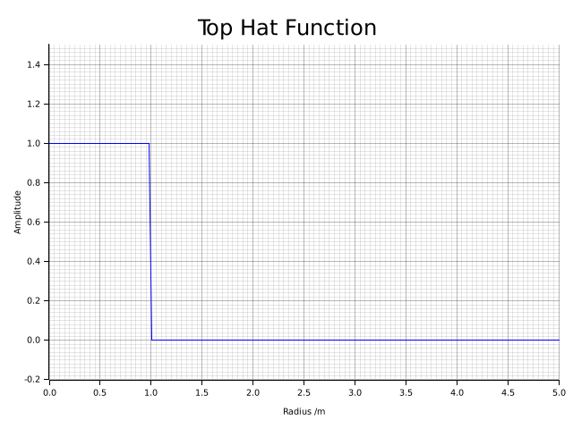
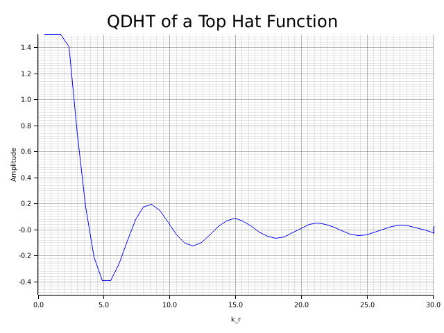
In this example (as in the Simple Example), we will check the band limit of a jinc function: \(f(r) = \frac{J_1(r)}{r}\). The (0 order) Hankel transform of this should be the top hat function. We'll also do the reverse: transforming a Top-Hat function to get a Jinc function.
In this case, we will use the simple, single shot functions. It should be noted though, this simplicity comes at an increased overhead, and for multiple transforms on the same grid, the approach in the Simple Example is recommended.
Here is the source code:
mod helper;
use amos_bessel_rs::bessel_j;
use hankrs::one_shot::qdht;
use ndarray::{Array1, Axis};

use crate::helper::plot_1d;

fn main() -> Result<(), Box<dyn std::error::Error>> {
    // --- PART 1: Jinc to Top-Hat ---
    // Create a grid for r points and calculate the jinc function.
    let r = Array1::linspace(0.0, 100.0, 1024);

    // The calculation fails at r = 0, so we have to set that manually to the limit of 1/2.
    let f = r.mapv(|rad| {
        if rad == 0.0 {
            0.5
        } else {
            bessel_j(1.0, rad).unwrap() / rad
        }
    });

    plot_1d(
        "one_shot_example_f.png",
        &r,
        &f,
        "Jinc Function",
        "Radius /m",
        "Amplitude",
        0.0..100.0,
        -0.2..0.6,
    )?;

    // Now take the Hankel transform using `qdht`:
    let (kr, ht) = qdht(r.clone(), &f, 0, Axis(0)).unwrap();

    // As expected, this is a top-hat function bandlimited to k<1, except for numerical error.
    plot_1d(
        "one_shot_example_ht.png",
        &kr,
        &ht,
        "Hankel Transform (Top Hat)",
        "Radial wavevector /m^-1",
        "Amplitude",
        0.0..5.0,
        -0.2..1.2,
    )?;

    // --- PART 2: Top-Hat to Jinc ---
    // Create a simple top-hat function
    let r2 = Array1::linspace(0.0, 5.0, 200);
    let f2 = r2.mapv(|rad| if rad < 1.0 { 1.0 } else { 0.0 });

    plot_1d(
        "one_shot_example_tophat.png",
        &r2,
        &f2,
        "Top Hat Function",
        "Radius /m",
        "Amplitude",
        0.0..5.0,
        -0.2..1.5,
    )?;

    // Transform
    let (kr2, ht2) = qdht(r2.clone(), &f2, 0, Axis(0)).unwrap();

    plot_1d(
        "one_shot_example_jinc.png",
        &kr2,
        &ht2,
        "QDHT of a Top Hat Function",
        "k_r",
        "Amplitude",
        0.0..30.0,
        -0.5..1.5,
    )?;

    Ok(())
}
Original Function (Jinc):
Hankel Transform (Top Hat):
Original Function (Top Hat):
Hankel Transform (Jinc):
Known Transforms
Below we demonstrate a range of known Hankel transform pairs from various sources.
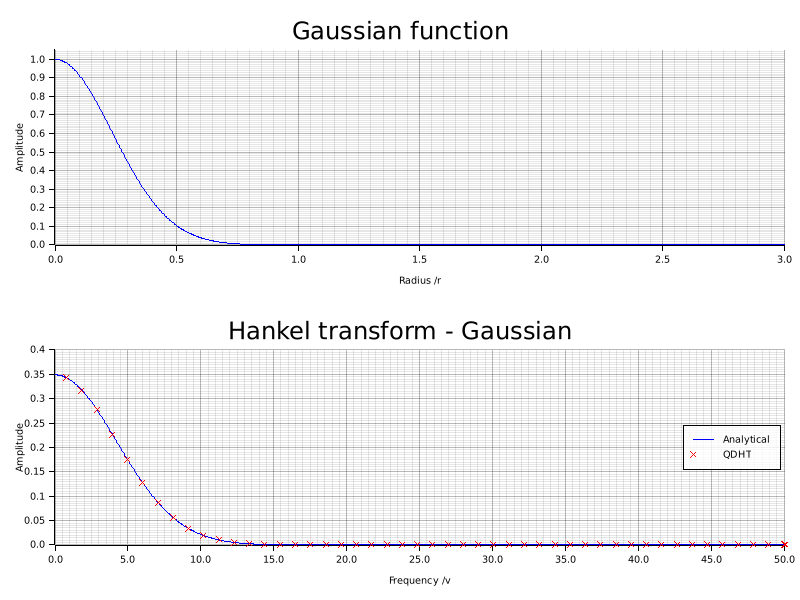
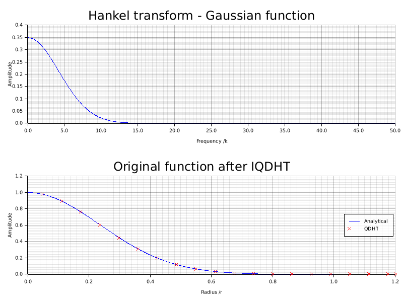
First we demonstrate the Gaussian function from Piessens [1] and its inverse transform.
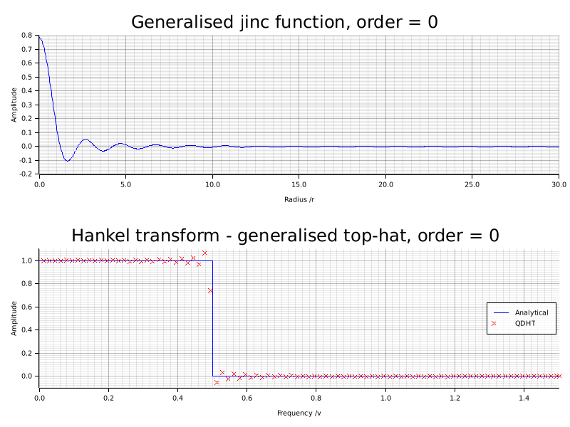
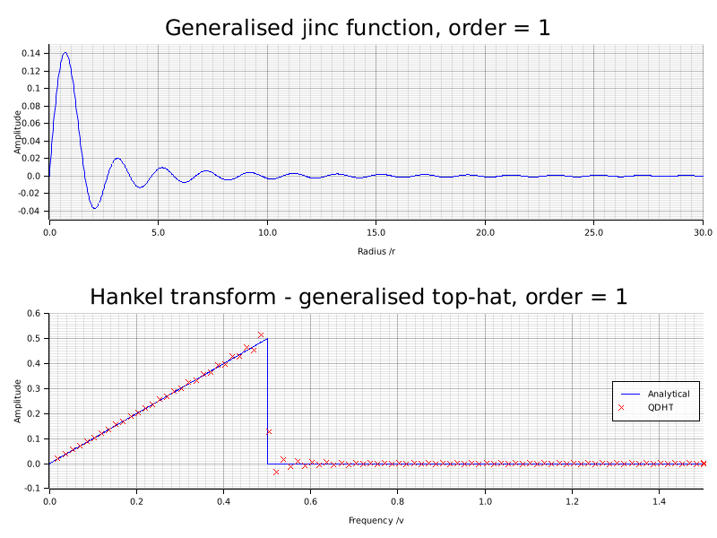
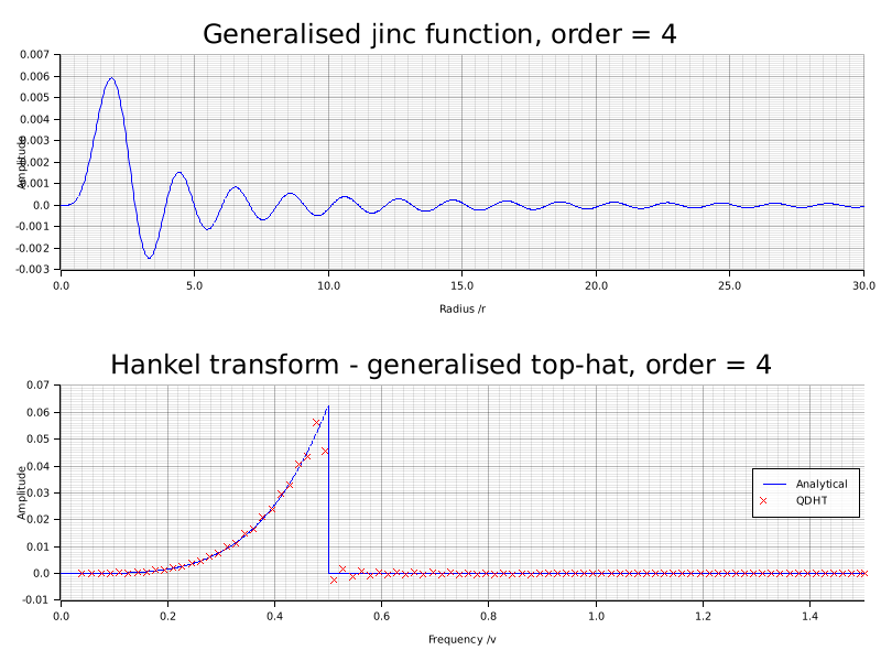
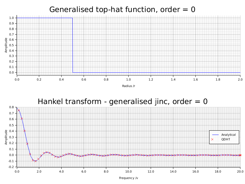
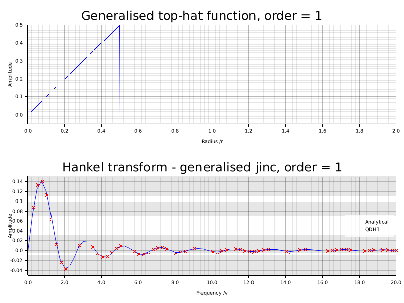
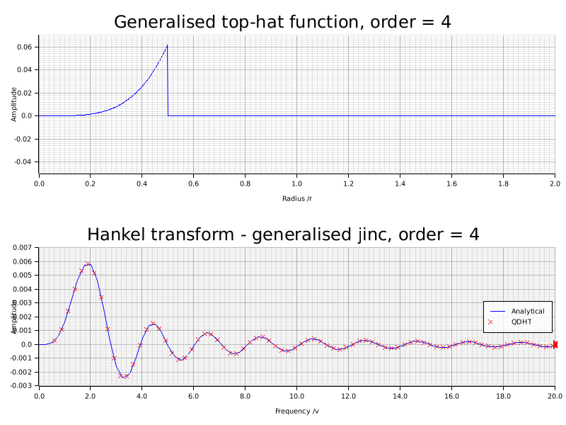
Then we check the "generalised top-hat" and "generalised jinc" functions from Guizar-Sicairos and Guitierrez-Vega [2].
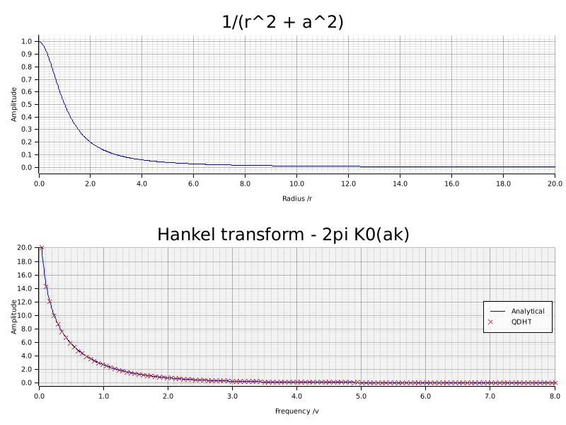
Finally, we look at the function \(f(r) = \frac{1}{r^2 + a^2}\), the Hankel transform of which is \(K_0(av)\), where \(K_0\) is the modified Bessel function of the second kind of order 0. [1]
[1] “Chapter 9: The Hankel Transform.” Piessens, R. in The Transforms and Applications Handbook: Second Edition. Ed. Alexander D. Poularikas. Boca Raton: CRC Press LLC, 2000 [2] "Computation of quasi-discrete Hankel transforms of the integer order for propagating optical wave fields" Manuel Guizar-Sicairos and Julio C. Guitierrez-Vega. J. Opt. Soc. Am. A 21 (1) 53-58 (2004)
mod helper;

use amos_bessel_rs::{bessel_j, bessel_k};
use hankrs::HankelTransform;
use hankrs::one_shot::{iqdht, qdht};
use helper::plot_1d_original_and_transform;
use ndarray::{Array1, ArrayRef1, Axis};
use std::f64::consts::PI;

fn generalised_top_hat(r: &ArrayRef1<f64>, a: f64, p: i32) -> Array1<f64> {
    r.mapv(|rad| if rad <= a { rad.powi(p) } else { 0.0 })
}

fn generalised_jinc(v: &ArrayRef1<f64>, a: f64, p: i32) -> Array1<f64> {
    v.mapv(|val| {
        if val != 0.0 {
            a.powi(p + 1) * bessel_j(f64::from(p) + 1.0, 2.0 * PI * a * val).unwrap() / val
        } else if p == -1 {
            f64::INFINITY
        } else if p == -2 {
            -PI
        } else if p == 0 {
            PI * a * a
        } else {
            0.0
        }
    })
}

#[allow(clippy::too_many_lines)]
fn main() -> Result<(), Box<dyn std::error::Error>> {
    // 1. Gaussian function
    // First we try a Gaussian function, the Hankel transform of which should also be Gaussian.
    //
    // Note the definition in Guizar-Sicairos varies from that used by
    // Piessens by a factor of 2\pi in both scaling of the argument (so we use
    // HankelTransform.kr rather than HankelTransform.v) and also scaling of the magnitude.
    let a = 3.0;
    let radius = Array1::linspace(0.0, 3.0, 1024);
    let f = radius.mapv(|r: f64| (-a * a * r * r).exp());
    let (kr, actual_ht) = qdht(radius.clone(), &f, 0, Axis(0)).unwrap();

    let kr_linear = Array1::linspace(0.0, 50.0, 1024);
    let expected_ht =
        kr_linear.mapv(|k: f64| 2.0 * PI * (1.0 / (2.0 * a * a)) * (-k * k / (4.0 * a * a)).exp());

    plot_1d_original_and_transform(
        "known_transforms_gaussian.png",
        &radius,
        &f,
        "Gaussian function",
        "Radius /r",
        "Amplitude",
        0.0..3.0,
        0.0..1.05,
        &kr_linear,
        &expected_ht,
        &kr,
        &actual_ht,
        "Analytical",
        "QDHT",
        "Hankel transform - Gaussian",
        "Frequency /v",
        "Amplitude",
        0.0..50.0,
        0.0..0.4,
    )?;

    // 2. Inverse Gaussian function
    // Now we repeat for the inverse transform
    let kr2 = Array1::linspace(0.0, 50.0, 1024);
    let ht = kr2.mapv(|k: f64| 2.0 * PI * (1.0 / (2.0 * a * a)) * (-k * k / (4.0 * a * a)).exp());
    let (r, actual_f) = iqdht(kr2.clone(), &ht, 0, Axis(0)).unwrap();

    let r_linear = Array1::linspace(0.0, 1.0, 1024);
    let expected_f = r_linear.mapv(|rad: f64| (-a * a * rad * rad).exp());

    plot_1d_original_and_transform(
        "known_transforms_inv_gaussian.png",
        &kr2,
        &ht,
        "Hankel transform - Gaussian function",
        "Frequency /k",
        "Amplitude",
        0.0..50.0,
        0.0..0.4,
        &r_linear,
        &expected_f,
        &r,
        &actual_f,
        "Analytical",
        "QDHT",
        "Original function after IQDHT",
        "Radius /r",
        "Amplitude",
        0.0..1.2,
        0.0..1.2,
    )?;

    // 3. Generalised jinc and top-hat
    // Next we define functions to calculate the generalised top-hat and jinc
    // functions, as defined by Guizar-Sicairos and Guitierrez-Vega.
    //
    // Note that for p=0 these become a standard top-hat and
    // jinc(r) = J_1(r)/r functions.
    let ylims3 = [
        (-0.2..0.8, -0.1..1.1),
        (-0.05..0.15, -0.1..0.6),
        (-0.003..0.007, -0.01..0.07),
    ];
    // For demonstration, we choose a = 0.5 and run the code for
    // orders 0, 1 and 4 plotting and checking the mean absolute error each time.
    // First check that the Hankel transform of the generalised jinc is calculated
    // correctly.
    let a_val = 0.5;
    let r3 = Array1::linspace(0.0, 30.0, 1024);
    for (i, &order) in [0, 1, 4].iter().enumerate() {
        let f = generalised_jinc(&r3, a_val, order);
        let (kr, actual_ht) = qdht(r3.clone(), &f, order, Axis(0)).unwrap();
        let v = kr.mapv(|k| k / (2.0 * PI));

        let v_linear = Array1::linspace(0.0, 1.5, 1024);
        let expected_ht = generalised_top_hat(&v_linear, a_val, order);

        let title_orig = format!("Generalised jinc function, order = {order}");
        let title_trans = format!("Hankel transform - generalised top-hat, order = {order}");
        plot_1d_original_and_transform(
            &format!("known_transforms_tophat_{order}.png"),
            &r3,
            &f,
            &title_orig,
            "Radius /r",
            "Amplitude",
            0.0..30.0,
            ylims3[i].0.clone(),
            &v_linear,
            &expected_ht,
            &v,
            &actual_ht,
            "Analytical",
            "QDHT",
            &title_trans,
            "Frequency /v",
            "Amplitude",
            0.0..1.5,
            ylims3[i].1.clone(),
        )?;
    }

    // 4. Generalised top-hat to jinc
    // Now we repeat but the other way round: the Hankel transform of the top-hat
    // function should be the jinc function.
    let r4 = Array1::linspace(0.0, 2.0, 1024);
    let ylims4 = [
        (-0.05..1.05, -0.2..0.8),
        (-0.05..0.5, -0.05..0.15),
        (-0.05..0.07, -0.003..0.007),
    ];

    for (i, &order) in [0, 1, 4].iter().enumerate() {
        let transformer = HankelTransform::new(order, 2.0, 1024).unwrap();
        let f = generalised_top_hat(&transformer.radius(), a_val, order);
        let actual_ht = transformer.qdht(&f, Axis(0));
        let v = transformer.frequency();

        let v_linear = Array1::linspace(0.0, transformer.max_frequency(), 1024);
        let expected_ht = generalised_jinc(&v_linear, a_val, order);

        let f_orig_linear = generalised_top_hat(&r4, a_val, order);
        let title_orig = format!("Generalised top-hat function, order = {order}");
        let title_trans = format!("Hankel transform - generalised jinc, order = {order}");
        plot_1d_original_and_transform(
            &format!("known_transforms_jinc_{order}.png"),
            &r4,
            &f_orig_linear,
            &title_orig,
            "Radius /r",
            "Amplitude",
            0.0..2.0,
            ylims4[i].0.clone(),
            &v_linear,
            &expected_ht,
            &v,
            &actual_ht,
            "Analytical",
            "QDHT",
            &title_trans,
            "Frequency /v",
            "Amplitude",
            0.0..20.0,
            ylims4[i].1.clone(),
        )?;
    }

    // 5. 1/(r^2 + a^2)
    // Now we investigate the function f(r) = 1/(r^2 + a^2),
    // the Hankel transform of which is K_0(av).
    //
    // Note again the scaling factor of 2\pi.
    let a5 = 1.0;
    let transformer = HankelTransform::new(0, 50.0, 1024).unwrap();
    let f5 = transformer.radius().mapv(|r| 1.0 / (r * r + a5 * a5));
    let actual_ht = transformer.qdht(&f5, Axis(0));
    let kr_grid = transformer.kr();

    let kr_linear = Array1::linspace(1e-6, 8.0, 1024);
    let expected_ht = kr_linear.mapv(|k| 2.0 * PI * bessel_k(0.0, a5 * k).unwrap());

    let r_linear = Array1::linspace(0.0, 20.0, 1024);
    let f5_linear = r_linear.mapv(|r| 1.0 / (r * r + a5 * a5));

    plot_1d_original_and_transform(
        "known_transforms_k0.png",
        &r_linear,
        &f5_linear,
        "1/(r^2 + a^2)",
        "Radius /r",
        "Amplitude",
        0.0..20.0,
        -0.05..1.05,
        &kr_linear,
        &expected_ht,
        &kr_grid,
        &actual_ht,
        "Analytical",
        "QDHT",
        "Hankel transform - 2pi K0(ak)",
        "Frequency /v",
        "Amplitude",
        0.0..8.0,
        -0.5..20.0,
    )?;

    Ok(())
}
Gaussian Function
Generalised Jinc to Top-Hat
Generalised Top-Hat to Jinc
K0 Function
Known Transforms — Spherical Hankel Transform
The spherical Hankel transform (SQDHT) is a variant of the QDHT designed for functions with spherical (3-D radial) symmetry. It computes
$$ H_\text{sph}^{(n)}{f}(k) = \int_0^\infty f(r)\; j_n(kr) \; r^2 \; dr $$
where \(j_n(x)\) is the nth-order spherical Bessel function of the first kind, defined as
$$ j_n(x) = \sqrt{\frac{\pi}{2x}} \; J_{n+\frac{1}{2}}(x) $$
Where \(J_n(x)\) is the Bessel function of the first kind. For n = 0, this reduces to \(j_0(x) = \sin(x)/x\) and hence
$$ H_\text{sph}^{(0)}{f}(k) = \int_0^\infty f(r) \, \frac{\sin(kr)}{kr} \, r^2 \, dr $$
While the zeroth order transform is demonstrated below, the HankelTransform object can be used to compute
transforms of any integer order.
A HankelTransform configured for spherical symmetry can be created with
HankelTransform::new_spherical(order, max_radius, n_points).
Below we verify two well-known transform pairs against their analytical results.
mod helper;

use hankrs::HankelTransform;
use helper::plot_1d_original_and_transform;
use ndarray::{Array1, Axis};
use std::f64::consts::PI;

fn main() -> Result<(), Box<dyn std::error::Error>> {
    // 1. Spherical Gaussian transform
    //
    // The order-0 spherical Hankel transform of a Gaussian f(r) = exp(-a*r^2) has the
    // analytical result:
    //
    //   H_sph{ f(r) }(k) = (sqrt(pi) / (4 * a^(3/2))) * exp(-k^2 / (4a))
    //
    // We demonstrate this for a = 2.0.
    let a = 2.0_f64;
    let r_max = 20.0;
    let n_points = 250;

    let transformer = HankelTransform::new_spherical(0, r_max, n_points).unwrap();

    let function: Array1<f64> = transformer.radius().mapv(|r| (-a * r.powi(2)).exp());

    let actual_transform = transformer.qdht(&function, Axis(0));
    let kr = transformer.kr();

    // Dense analytical curve for plotting
    let kr_linear = Array1::linspace(0.0, *kr.last().unwrap(), 1024);
    let expected_transform = kr_linear.mapv(|k| {
        let prefactor = PI.sqrt() / (4.0 * a.powf(1.5));
        prefactor * (-(k.powi(2)) / (4.0 * a)).exp()
    });

    // Dense original function for plotting
    let r_linear = Array1::linspace(0.0, r_max * 0.5, 1024);
    let f_linear = r_linear.mapv(|r| (-a * r.powi(2)).exp());

    plot_1d_original_and_transform(
        "spherical_known_transforms_gaussian.png",
        &r_linear,
        &f_linear,
        "Gaussian function: exp(-r²)",
        "Radius r",
        "Amplitude",
        0.0..4.0,
        -0.05..1.05,
        &kr_linear,
        &expected_transform,
        &kr,
        &actual_transform,
        "Analytical",
        "SQDHT",
        "Spherical Hankel transform - Gaussian",
        "Wavenumber k",
        "Amplitude",
        0.0..10.0,
        -0.01..0.2,
    )?;

    // 2. Spherical top-hat transform
    //
    // The order-0 spherical Hankel transform of a top-hat function f(r) = 1 for r < a,
    // 0 otherwise, has the analytical result:
    //
    //   H_sph{ f(r) }(k) = (sin(ka) - ka*cos(ka)) / k^3
    //
    // We demonstrate this for a = 0.5
    let a_hat = 0.5_f64;
    let r_max_hat = 20.0;
    let n_points_hat = 1000;

    let transformer_hat = HankelTransform::new_spherical(0, r_max_hat, n_points_hat).unwrap();

    // Build top-hat on the QDHT grid; snap `a` to the nearest grid point
    let function_hat: Array1<f64> = transformer_hat
        .radius()
        .mapv(|r| if r < a_hat { 1.0 } else { 0.0 });

    // Snap a to the nearest grid sample to remove discretisation error in the comparison
    let actual_a = transformer_hat
        .radius()
        .iter()
        .rposition(|&r| r < a_hat)
        .map_or(a_hat, |idx| transformer_hat.radius()[idx]);

    let actual_transform_hat = transformer_hat.qdht(&function_hat, Axis(0));
    let kr_hat = transformer_hat.kr();

    // Dense analytical curve for plotting
    let kr_hat_linear = Array1::linspace(1e-6, *kr_hat.last().unwrap(), 1024);
    let expected_transform_hat = kr_hat_linear
        .mapv(|k| { (k * actual_a).sin() - k * actual_a * (k * actual_a).cos() } / k.powi(3));

    // Dense original function for plotting
    let r_hat_linear = Array1::linspace(0.0, 3.0, 1024);
    let f_hat_linear = r_hat_linear.mapv(|r| if r < a_hat { 1.0 } else { 0.0 });

    plot_1d_original_and_transform(
        "spherical_known_transforms_tophat.png",
        &r_hat_linear,
        &f_hat_linear,
        "Top-hat function: 1 for r < a",
        "Radius r",
        "Amplitude",
        0.0..2.0,
        -0.1..1.2,
        &kr_hat_linear,
        &expected_transform_hat,
        &kr_hat,
        &actual_transform_hat,
        "Analytical",
        "SQDHT",
        "Spherical Hankel transform - Top-Hat",
        "Wavenumber k",
        "Amplitude",
        0.0..30.0,
        -0.02..0.05,
    )?;

    Ok(())
}
Gaussian Function
The order-0 spherical Hankel transform of the Gaussian \(f(r) = e^{-ar^2}\) is
$$H_\text{sph}{e^{-ar^2}}(k) = \frac{\sqrt{\pi}}{4\, a^{3/2}}\, e^{-k^2 / 4a}$$
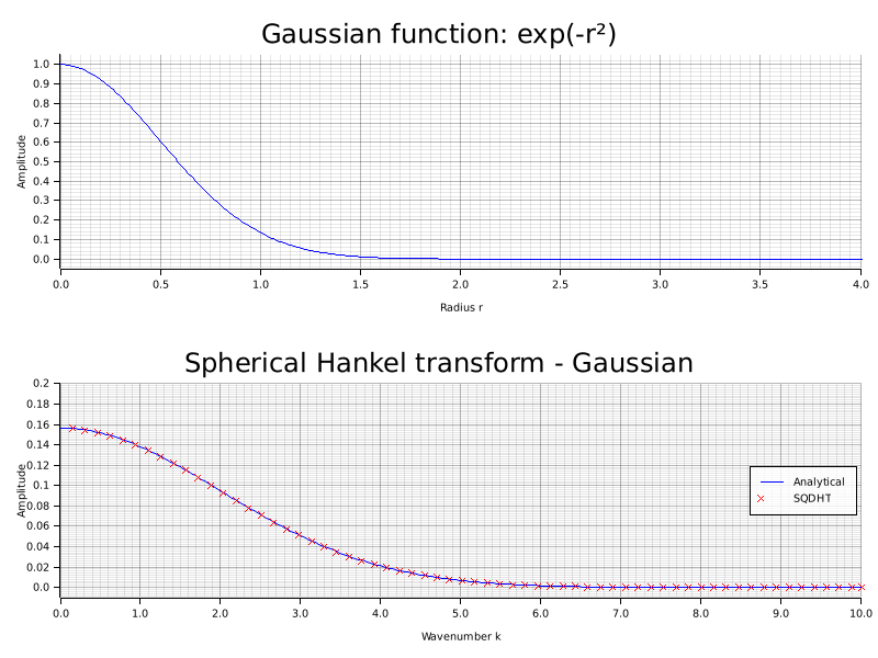
The SQDHT (circles) closely follows the analytical result (solid line) across the entire wavenumber range.
Top-Hat Function
The order-0 spherical Hankel transform of the top-hat \(f(r) = 1\) for \(r < a\), \(0\) otherwise, is
$$H_\text{sph}{f}(k) = \frac{\sin(ka) - ka\cos(ka)}{k^3}$$
This is the 3-D analogue of the familiar jinc function that arises in the standard (2-D radially-symmetric) Hankel transform.
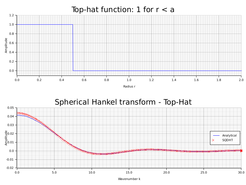
The oscillatory decay of the transform reflects the sharp edge of the top-hat, again in excellent agreement with the analytical formula.
Literature Comparison
This example is a comparison of hankrs against results from the original publication of the quasi-discrete Hankel transform method:
"Computation of quasi-discrete Hankel transforms of the integer order for propagating optical wave fields" Manuel Guizar-Sicairos and Julio C. Guitierrez-Vega J. Opt. Soc. Am. A 21 (1) 53-58 (2004)
mod helper;
use amos_bessel_rs::bessel_j;
use approx::assert_abs_diff_eq;
use hankrs::HankelTransform;
use ndarray::{Array1, ArrayRef1, Axis};
use std::f64::consts::PI;

use crate::helper::{plot_1d, plot_1d_compare};

fn sinc(x: &ArrayRef1<f64>) -> Array1<f64> {
    x.mapv(|val| if val == 0.0 { 1.0 } else { val.sin() / val })
}

/// Equation 12 of Guizar
fn hankel_transform_of_sinc(v: &ArrayRef1<f64>, gamma: f64, p: i32) -> Array1<f64> {
    v.mapv(|val| {
        if val < gamma {
            val.powi(p) * (f64::from(p) * PI / 2.0).cos()
                / (2.0
                    * PI
                    * gamma
                    * (gamma * gamma - val * val).sqrt()
                    * (gamma + (gamma * gamma - val * val).sqrt()).powi(p))
        } else {
            (f64::from(p) * (gamma / val).asin()).sin()
                / (2.0 * PI * gamma * (val * val - gamma * gamma).sqrt())
        }
    })
}

#[allow(clippy::cast_precision_loss, clippy::too_many_lines)]
fn main() -> Result<(), Box<dyn std::error::Error>> {
    // 1. Sinc function and dynamical error (Figure 1 of Guizar)
    // First we will reproduce figure 1 of Guizar-Sicairos & Guitierrez-Vega
    // Now plot the values of the hankel transform and the dynamical error as in figure 1
    // for order 1 and 4
    for &p in &[1, 4] {
        let transformer = HankelTransform::new(p, 3.0, 256).unwrap();
        let gamma = 5.0;
        let r = transformer.radius();
        let func = sinc(&r.mapv(|rad| 2.0 * PI * gamma * rad));
        let v = transformer.kr().mapv(|k| k / (2.0 * PI));
        let expected_ht = hankel_transform_of_sinc(&v, gamma, p);
        let ht = transformer.qdht(&func, Axis(0));

        let v_linear = Array1::linspace(0.0, 10.0, 1024);
        let expected_ht_linear = hankel_transform_of_sinc(&v_linear, gamma, p);

        let ht_max = ht.iter().copied().fold(f64::NEG_INFINITY, f64::max);
        let dynamical_error = ht
            .iter()
            .zip(expected_ht.iter())
            .map(|(&h, &e)| 20.0 * ((e - h).abs() / ht_max).log10())
            .collect::<Array1<f64>>();

        let title = format!("Hankel Transform, p={p}");
        plot_1d_compare(
            &format!("lit_comp_sinc_ht_{p}.png"),
            &v_linear,
            &expected_ht_linear,
            &v,
            &ht,
            "Analytical",
            "QDHT",
            &title,
            "Frequency /v",
            "Amplitude",
            0.0..10.0,
            -0.05..0.05,
        )?;

        plot_1d(
            &format!("lit_comp_sinc_error_{p}.png"),
            &v,
            &dynamical_error,
            "Dynamical error",
            "Frequency /v",
            "Error /dB",
            0.0..10.0,
            -150.0..0.0,
        )?;
    }

    // 2. Figure 3 and Table 1 of Guizar
    // Now we will reproduce figure 3 and confirm we can replicate
    // the errors in the top half of table 1.
    let p = 4;
    let a = 1.0;

    // We'll just do 1024 points for the example
    let transformer = HankelTransform::new(p, 2.0, 1024).unwrap();
    let r = transformer.radius();
    let func = r.mapv(|rad| if rad <= a { rad.powi(p) } else { 0.0 });

    let v = transformer.kr().mapv(|k| k / (2.0 * PI));
    let expected_ht = v.mapv(|v_val| {
        if v_val == 0.0 {
            0.0 // handled implicitly in jinc
        } else {
            a.powi(p + 1) * bessel_j(f64::from(p) + 1.0, 2.0 * PI * a * v_val).unwrap() / v_val
        }
    });

    let v_linear = Array1::linspace(0.0, 10.0, 1024);
    let expected_ht_linear = v_linear.mapv(|v_val| {
        if v_val == 0.0 {
            0.0 // handled implicitly in jinc
        } else {
            a.powi(p + 1) * bessel_j(f64::from(p) + 1.0, 2.0 * PI * a * v_val).unwrap() / v_val
        }
    });

    let ht = transformer.qdht(&func, Axis(0));
    let retrieved_func = transformer.iqdht(&ht, Axis(0));

    let v = transformer.kr().mapv(|k| k / (2.0 * PI));
    plot_1d_compare(
        "lit_comp_fig3_ht.png",
        &v_linear,
        &expected_ht_linear,
        &v,
        &ht,
        "Analytical",
        "QDHT",
        &format!("Hankel transform f_2(v), order {p}"),
        "Frequency /v",
        "Amplitude",
        0.0..10.0,
        -0.2..1.0,
    )?;

    let r_linear = Array1::linspace(0.0, 2.0, 1024);
    let func_linear = r_linear.mapv(|rad| if rad <= a { rad.powi(p) } else { 0.0 });

    plot_1d_compare(
        "lit_comp_fig3_retrieved.png",
        &r_linear,
        &func_linear,
        &r,
        &retrieved_func,
        "Analytical",
        "QDHT+iQDHT",
        "Round-trip QDHT vs analytical function",
        "Radius /r",
        "Amplitude",
        0.0..2.0,
        -0.2..1.2,
    )?;

    // Now check that the error is the same as that given in Table 1
    // Check that the error is low, as they do in the paper. Numbers are estimated from their graphs
    let error_2: f64 = expected_ht
        .iter()
        .zip(ht.iter())
        .map(|(&e, &h)| (e - h).abs())
        .sum::<f64>()
        / ht.len() as f64;
    let error_1: f64 = func
        .iter()
        .zip(retrieved_func.iter())
        .map(|(&f_val, &r_val)| (f_val - r_val).abs())
        .sum::<f64>()
        / func.len() as f64;

    println!("**1024 Points:**");
    println!("- Error in Hankel transform is {error_2:.2e}");
    println!("- Error in reconstructed function is {error_1:.2e}");

    assert_abs_diff_eq!(error_2, 4.8e-5, epsilon = 1e-6);
    // Note that Guizar-Sicairos & Guitierrez-Vega got 2.7e-14, so ours is slightly lower
    assert_abs_diff_eq!(error_1, 2.15e-14, epsilon = 1e-15);

    // Now repeat for 512 points
    let transformer_512 = HankelTransform::new(p, 2.0, 512).unwrap();
    let r_512 = transformer_512.radius();
    let func_512 = r_512.mapv(|rad| if rad <= a { rad.powi(p) } else { 0.0 });

    let v_512 = transformer_512.kr().mapv(|k| k / (2.0 * PI));
    let expected_ht_512 = v_512.mapv(|v_val| {
        if v_val == 0.0 {
            0.0 // handled implicitly in jinc
        } else {
            a.powi(p + 1) * bessel_j(f64::from(p) + 1.0, 2.0 * PI * a * v_val).unwrap() / v_val
        }
    });

    let ht_512 = transformer_512.qdht(&func_512, Axis(0));
    let retrieved_func_512 = transformer_512.iqdht(&ht_512, Axis(0));

    let error_2_512: f64 = expected_ht_512
        .iter()
        .zip(ht_512.iter())
        .map(|(&e, &h)| (e - h).abs())
        .sum::<f64>()
        / ht_512.len() as f64;
    let error_1_512: f64 = func_512
        .iter()
        .zip(retrieved_func_512.iter())
        .map(|(&f_val, &r_val)| (f_val - r_val).abs())
        .sum::<f64>()
        / func_512.len() as f64;

    println!("\n**512 Points:**");
    println!("- Error in Hankel transform is {error_2_512:.2e}");
    println!("- Error in reconstructed function is {error_1_512:.2e}");

    // Note the below is 10 times smaller than
    // Guizar-Sicairos & Guitierrez-Vega (1.3e-3)
    assert_abs_diff_eq!(error_2_512, 1.3e-4, epsilon = 1e-5);
    assert_abs_diff_eq!(error_1_512, 2.2e-13, epsilon = 1e-14);

    Ok(())
}
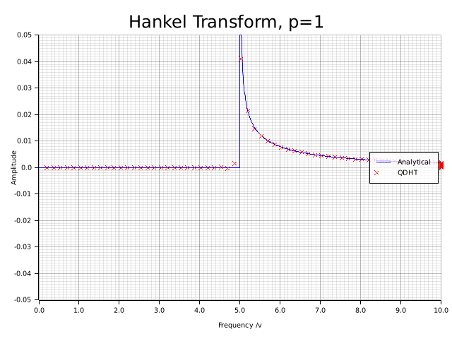
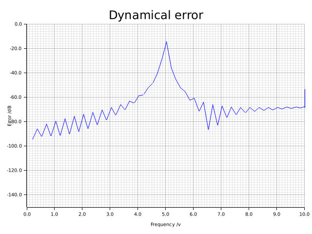
Figure 1: Hankel Transform of a Sinc Function
We reproduce figure 1 of Guizar-Sicairos & Guitierrez-Vega, showing the Hankel transform of a sinc function and the dynamical error, for orders 1 and 4.
Order 1
Order 4
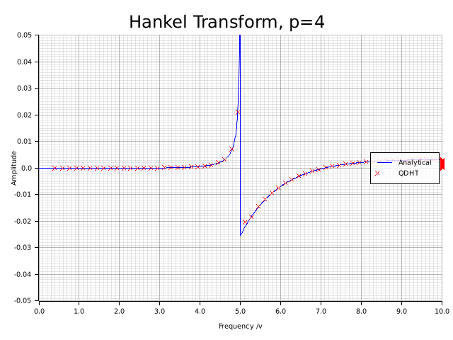
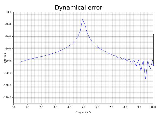
Figure 3: Round-Trip Transformation
We reproduce figure 3, applying a forward transform and an inverse transform (round-trip), demonstrating high fidelity.
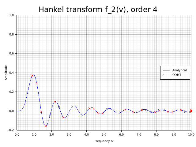
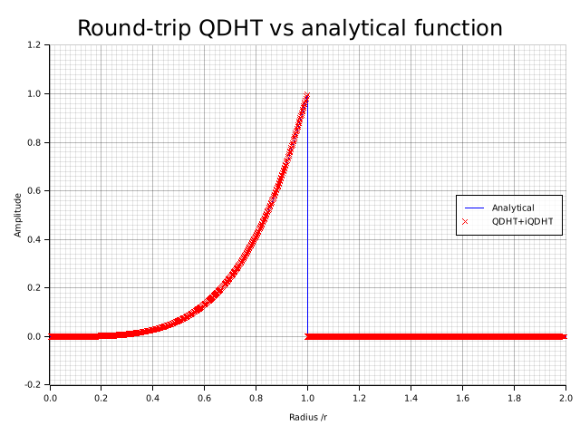
Table 1: Error Calculations
The calculated errors for the Hankel transform and the reconstructed function match the values given in Table 1 of the Guizar-Sicairos & Guitierrez-Vega paper.
1024 Points:
- Error in Hankel transform is 4.81e-5
- Error in reconstructed function is 2.12e-14
512 Points:
- Error in Hankel transform is 1.35e-4
- Error in reconstructed function is 2.26e-13
Complex Beam Propagation
To demonstrate the full power of HankelTransform with complex values, we will give an example of propagating a radially-symmetric beam using the beam propagation method.
In this case, it will be a simple Gaussian beam propagating away from focus and diverging. We'll utilize the <T: HankelScalar> generic trait to perform the QDHT directly on a Complex64 array.
First we will use a loop over the \(z\) position, and then we will demonstrate that the HankelTransform methods can perfectly vectorize the \(z\)-axis propagation by processing multiple columns natively.
Here is the source code:
mod helper;
use hankrs::HankelTransform;
use ndarray::{Array1, Array2, Axis};
use num_complex::Complex64;
use std::f64::consts::PI;

use crate::helper::{imagesc, plot_1d, plot_1d_compare};

#[allow(clippy::too_many_lines, clippy::similar_names)]
fn main() -> Result<(), Box<dyn std::error::Error>> {
    let nr = 1024;
    let r_max = 5e-3;
    let r = Array1::linspace(0.0, r_max, nr);

    let nz = 200;
    let z_max = 0.1;
    let z = Array1::linspace(0.0, z_max, nz);

    let dr = 100e-6;
    let lambda_ = 488e-9;
    let k0 = 2.0 * PI / lambda_;

    // Set up a HankelTransform object, telling it the order (0) and the radial grid.
    let transformer = HankelTransform::new_from_r_grid(0, r.clone()).unwrap();

    // Set up the electric field profile at z = 0, and resample onto the correct radial grid
    // (transformer.radius()) as required for the QDHT.
    let er_real = helper::gauss1d(&r, 0.0, dr);
    let er: Array1<Complex64> = er_real.mapv(|v| Complex64::new(v, 0.0));
    let er_h = transformer.to_transform_r(&er).unwrap();

    // Convert from physical field to physical wavevector
    let ekr_h = transformer.qdht(&er_h, Axis(0));

    // Plotting
    // Plot the initial field and radial wavevector distribution (given by the
    // Hankel transform)

    let r_mm = r.mapv(|val| val * 1e3);
    let transformer_r_mm = transformer.radius().mapv(|val| val * 1e3);

    let abs_er = er.mapv(|c| c.norm_sqr());
    let abs_er_h = er_h.mapv(|c| c.norm_sqr());

    plot_1d_compare(
        "usage_example_initial_field.png",
        &r_mm,
        &abs_er,
        &transformer_r_mm,
        &abs_er_h,
        "|E(r)|^2",
        "|E(H.r)|^2",
        "Initial electric field distribution",
        "Radial co-ordinate (r) /mm",
        "Field intensity /arb.",
        0.0..1.0,
        0.0..1.0,
    )?;

    let abs_ekr_h = ekr_h.mapv(|c| c.norm_sqr());
    let ht_max = abs_ekr_h.iter().copied().fold(f64::NEG_INFINITY, f64::max);
    plot_1d(
        "usage_example_k_vector.png",
        &transformer.kr(),
        &abs_ekr_h,
        "Radial wave-vector distribution",
        "Radial wave-vector (k_r) /rad m^-1",
        "Field intensity /arb.",
        0.0..30000.0,
        0.0..ht_max * 1.05,
    )?;

    // Propagate the beam - loop
    // Do the propagation in a loop over z
    // Pre-allocate an array for field as a function of r and z
    let mut erz = Array2::<Complex64>::zeros((nr, nz));
    let kz = transformer
        .kr()
        .mapv(|kr_val| (k0 * k0 - kr_val * kr_val).sqrt());

    for (i, &z_loop) in z.iter().enumerate() {
        let phi_z = kz.mapv(|kz_val| kz_val * z_loop); // Propagation phase
        let ekr_hz = ndarray::Zip::from(&ekr_h)
            .and(&phi_z)
            .map_collect(|&ekr, &phi| ekr * Complex64::new(0.0, phi).exp()); // Apply propagation
        let er_hz = transformer.iqdht(&ekr_hz, Axis(0)); // iQDHT
        let erz_slice = transformer.to_original_r(&er_hz).unwrap(); // Interpolate output
        erz.column_mut(i).assign(&erz_slice);
    }
    let irz = erz.mapv(|c| c.norm_sqr());

    let z_mm = z.mapv(|val| val * 1e3);
    let r_mm = r.mapv(|val| val * 1e3);

    // Now plot an image showing the intensity as a function of
    // radius and propagation distance.

    imagesc(
        "usage_example_irz.png",
        &z_mm,
        &r_mm,
        &irz,
        "Radial field intensity",
        "Propagation distance (z) /mm",
        "Radial position (r) /mm",
        0.0..1.0,
    )?;

    // The plot above shows a reduction of intensity with z, but it is
    // bit difficult to see the beam growing in r. To show that, let's
    // plot the intensity normalised such that the peak intensity at each z
    // coordinate is the same.
    let mut irz_norm = irz.clone();
    for i in 0..nz {
        let peak = irz_norm
            .column(i)
            .iter()
            .copied()
            .fold(f64::NEG_INFINITY, f64::max);
        if peak > 0.0 {
            let mut col = irz_norm.column_mut(i);
            col.mapv_inplace(|v| v / peak);
        }
    }

    imagesc(
        "usage_example_irz_norm.png",
        &z_mm,
        &r_mm,
        &irz_norm,
        "Normalised Radial field intensity",
        "Propagation distance (z) /mm",
        "Radial position (r) /mm",
        0.0..1.0,
    )?;

    // Propagate the beam - vectorised approach
    // We can also propagate it entirely within Hankel space without having to drop out in a loop!
    // By creating a 2D array of the wave propagation, we can apply the inverse QDHT
    // down the 0th axis in a single vectorized shot.
    let ekr_hz_vec = Array2::from_shape_fn((nr, nz), |(i, j)| {
        ekr_h[i] * Complex64::new(0.0, kz[i] * z[j]).exp()
    });

    let er_hz_vec = transformer.iqdht(&ekr_hz_vec, Axis(0));
    let erz_vec = transformer.to_original_r_nd(&er_hz_vec, Axis(0)).unwrap();

    let irz_vec = erz_vec.mapv(|c| c.norm_sqr());

    // Now plot the result to check it is the same as the loop approach
    imagesc(
        "usage_example_irz_vec.png",
        &z_mm,
        &r_mm,
        &irz_vec,
        "Radial field intensity as a function of propagation for annular beam",
        "Propagation distance (z) /mm",
        "Radial position (r) /mm",
        0.0..1.0,
    )?;

    #[allow(clippy::cast_precision_loss)]
    let total_n = (nr * nz) as f64;
    // Assert the two approaches produce the same intensity
    // Assert matches
    let error: f64 = irz
        .iter()
        .zip(irz_vec.iter())
        .map(|(&a, &b)| (a - b).abs())
        .sum::<f64>()
        / total_n;
    assert!(error < 1e-10);

    Ok(())
}
Initial Electric Field Distribution:
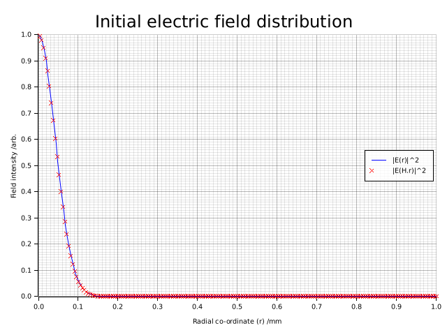
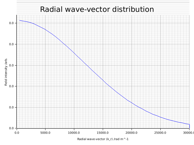
Radial Field Intensity as a Function of Propagation:
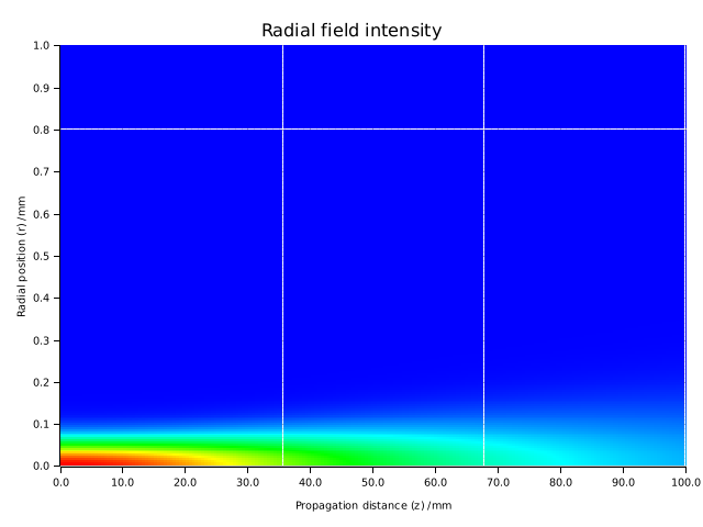
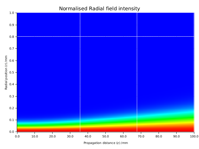
Because the intensity drops as the beam expands, it might be difficult to clearly see the beam growing in \(r\). To show that better, let's plot the intensity normalised such that the peak intensity at each \(z\) coordinate is identical.
Normalised Radial Field Intensity:
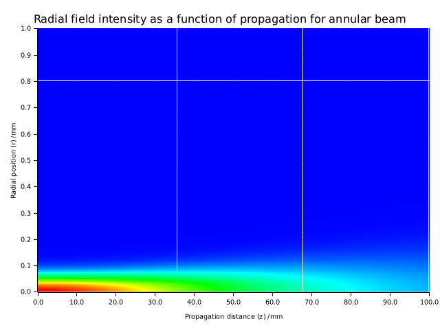
Vectorised Approach Match:
We can also verify that propagating it using the vectorised array matches the loop exactly.
Speed Comparison: Single-Shot vs Reusable Objects
For a simple case, there are convenience functions (hankrs::one_shot::qdht and iqdht) which can be used to calculate the transform of a function without needing to manually manage a state object.
However, these functions come with heavy internal overhead because they completely re-calculate all of the Bessel roots and transformation matrices on every single call. To demonstrate this overhead, we will use the exact same beam-propagation application as in our Complex Beam Propagation example, and time the difference between generating a state machine once vs relying on one_shot.
Here is the source code:
mod helper;
use hankrs::one_shot::{iqdht, qdht};
use hankrs::{HankelScalar, HankelTransform};
use ndarray::{Array1, Array2, ArrayRef1, Axis};
use num_complex::Complex64;
use std::f64::consts::PI;
use std::time::Instant;

use crate::helper::imagesc;

// Speed of single-shot vs reuse of a HankelTransform object
//
// For a simple case there are two simple forward and inverse functions which can be used to calculate the
// Hankel transform of a function sampled at an arbitrary set of points in radius / wave-number space.
// Here we will use the same example application as the usage_example:
// a beam-propagation method propagation of a radially-symmetric Gaussian beam.
fn propagate_using_object(
    r: &ArrayRef1<f64>,
    field: &ArrayRef1<Complex64>,
    nr: usize,
    nz: usize,
    z: &ArrayRef1<f64>,
    k0: f64,
) -> Array2<f64> {
    let transformer = HankelTransform::new_from_r_grid(0, r.to_owned()).unwrap();
    let field_for_transform = transformer.to_transform_r(field).unwrap(); // Resampled field
    let hankel_transform = transformer.qdht(&field_for_transform, Axis(0));

    let mut propagated_field = Array2::<Complex64>::zeros((nr, nz));
    let kz = transformer
        .kr()
        .mapv(|kr_val| (k0 * k0 - kr_val * kr_val).sqrt());

    for (n, &z_loop) in z.iter().enumerate() {
        let phi_z = kz.mapv(|kz_val| kz_val * z_loop); // Propagation phase
        let hankel_transform_at_z = ndarray::Zip::from(&hankel_transform)
            .and(&phi_z)
            .map_collect(|&ekr, &phi| ekr * Complex64::new(0.0, phi).exp()); // Apply propagation
        let field_at_z = transformer.iqdht(&hankel_transform_at_z, Axis(0)); // iQDHT
        let field_slice = transformer.to_original_r(&field_at_z).unwrap(); // Interpolate output
        propagated_field.column_mut(n).assign(&field_slice);
    }
    propagated_field.mapv(|c| c.norm_sqr())
}

fn propagate_using_single_shot(
    r: &ArrayRef1<f64>,
    field: &ArrayRef1<Complex64>,
    nr: usize,
    nz: usize,
    z: &ArrayRef1<f64>,
    k0: f64,
) -> Array2<f64> {
    let (kr, hankel_transform) = qdht(r.to_owned(), field, 0, Axis(0)).unwrap();

    let mut propagated_field = Array2::<Complex64>::zeros((nr, nz));
    let kz = kr.mapv(|kr_val| (k0 * k0 - kr_val * kr_val).sqrt());

    for (n, &z_loop) in z.iter().enumerate() {
        let phi_z = kz.mapv(|kz_val| kz_val * z_loop);
        let hankel_transform_at_z = ndarray::Zip::from(&hankel_transform)
            .and(&phi_z)
            .map_collect(|&ekr, &phi| ekr * Complex64::new(0.0, phi).exp());
        let (r_transform, field_at_z) =
            iqdht(kr.clone(), &hankel_transform_at_z, 0, Axis(0)).unwrap();

        let field_slice = Complex64::spline(&r_transform, &field_at_z, r, Axis(0));
        propagated_field.column_mut(n).assign(&field_slice);
    }
    propagated_field.mapv(|c| c.norm_sqr())
}

fn main() -> Result<(), Box<dyn std::error::Error>> {
    let nr = 1024;
    let r_max = 5e-3;
    let r = Array1::linspace(0.0, r_max, nr);

    let nz = 100;
    let z_max = 0.1;
    let z = Array1::linspace(0.0, z_max, nz);

    let dr = 100e-6;
    let lambda_ = 488e-9;
    let k0 = 2.0 * PI / lambda_;

    let field_real = helper::gauss1d(&r, 0.0, dr); // Initial field
    let field: Array1<Complex64> = field_real.mapv(|v| Complex64::new(v, 0.0));

    // Now we need two functions that propagate the beam in two ways (giving the same answer).
    // The first will use single shot, the second will use a HankelTransform object.
    // Below we will run each of them in turn and compare the speed.

    // Now run and time the two functions:
    let start = Instant::now();
    let single_shot_intensity = propagate_using_single_shot(&r, &field, nr, nz, &z, k0);
    let duration = start.elapsed();
    println!(
        "Single shot propagation took {:.2?} s",
        duration.as_secs_f64()
    );

    let start = Instant::now();
    let object_intensity = propagate_using_object(&r, &field, nr, nz, &z, k0);
    let duration = start.elapsed();
    println!("Object propagation took {:.2?} s", duration.as_secs_f64());

    // The single shot approach takes a *lot* longer!
    // Plot the two results to check they are the same:

    let z_mm = z.mapv(|val| val * 1e3);
    let r_mm = r.mapv(|val| val * 1e3);

    imagesc(
        "speed_usage_single_shot.png",
        &z_mm,
        &r_mm,
        &single_shot_intensity,
        "Single Shot Output",
        "Propagation distance (z) /mm",
        "Radial position (r) /mm",
        0.0..1.0,
    )?;

    imagesc(
        "speed_usage_object.png",
        &z_mm,
        &r_mm,
        &object_intensity,
        "Object Output",
        "Propagation distance (z) /mm",
        "Radial position (r) /mm",
        0.0..1.0,
    )?;

    Ok(())
}
The Results
If we compile and run this in release mode via cargo run --release --example speed_usage_example, the performance gap is monumental:
Single shot propagation took 2.11 s Object propagation took 0.26 s
The struct-based approach completes in a fraction of a second, yielding roughly a ~50x speedup just by holding onto the HankelTransform struct. When performing multiple identical QDHT operations, it is significantly faster to maintain and reuse HankelTransform objects.
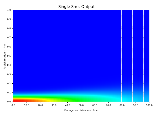
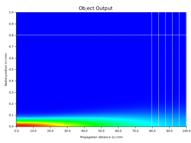
To verify they output exactly the same data, we can plot the resulting beam propagation for both approaches: